GHOST | Hyperspectral Segmentation

New Release v0.1.7 PyPI →

Adds ghost convert_to_mat — convert ENVI, TIFF, GeoTIFF, and HDF5/NetCDF hyperspectral images to .mat format. Auto-detects format from extension, preserves all metadata (CRS, wavelengths, band names) in a JSON sidecar, and supports ground truth in .mat, .png, .tif, or .hdr.

$ Terminal

pip install ghost-hsi[convert]

ghost convert_to_mat \
  --img image.hdr \
  --gt  labels.tif \
  --out-dir converted/

What does "generalizable" actually mean here?

For a hyperspectral model to work across different scenes without retraining, a few things need to be true. Here's where GHOST currently stands.

✓

Data Agnostic

Band count, class count, and spatial dimensions are all read from the file at runtime. Nothing is hardcoded. Same binary on Indian Pines, LUSC, and Mars CRISM.

✓

Band Count Agnostic

Works on 3 bands or 400+. Same pipeline, any sensor resolution, no configuration needed.

✓

Sensor Agnostic

Remote sensing, medical pathology, planetary science — no format-specific code paths, no domain-specific preprocessing.

⚠

Spectral-Only Context Still in progress

For true scene-to-scene transfer, the model needs to classify each pixel from its spectrum alone — no spatial context from neighbors. We're not there yet.

Results.

Tested on standard HSI benchmarks. These numbers are from single-scene pixel-level evaluation, which is the standard for these datasets but doesn't say much about real-world generalization. Expect roughly ±1% variance between runs due to random splits and seed sensitivity. Take them accordingly.

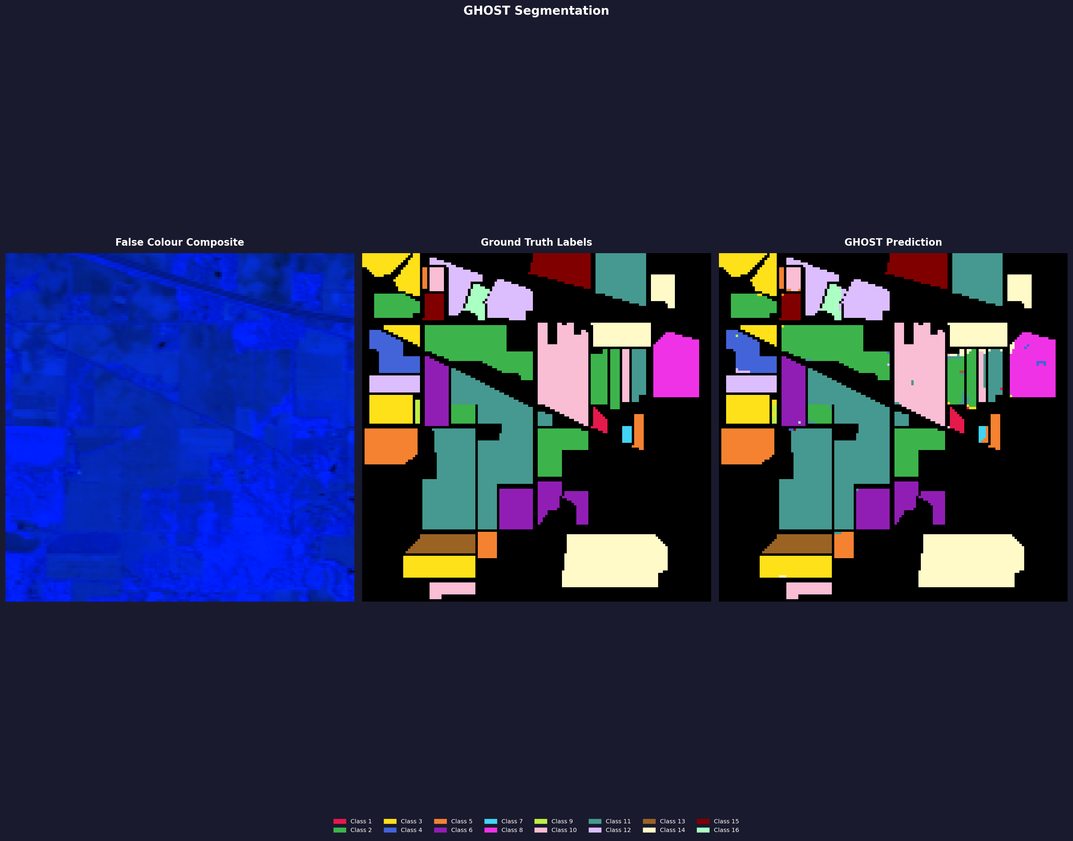
Indian Pines

200 bands · 16 classes · Remote Sensing (AVIRIS)

Metrics

Config	OA (%)	mIoU	Kappa
64 / 16	98.16	0.9071	0.9790
32 / 8	97.20	0.8030	0.9681

Config

Base / Num Filters	GPU	Time
64 / 16	RTX 3050 (laptop)	2h 20m
32 / 8	RTX 3050 (laptop)	1h 17m

Standard pixel-level split — 20% train, 10% val, 70% test, seed 42, forest routing, dice loss. The image shown is the 64/16 run. Both runs use the same scene — evaluation is inflated relative to cross-scene generalization.

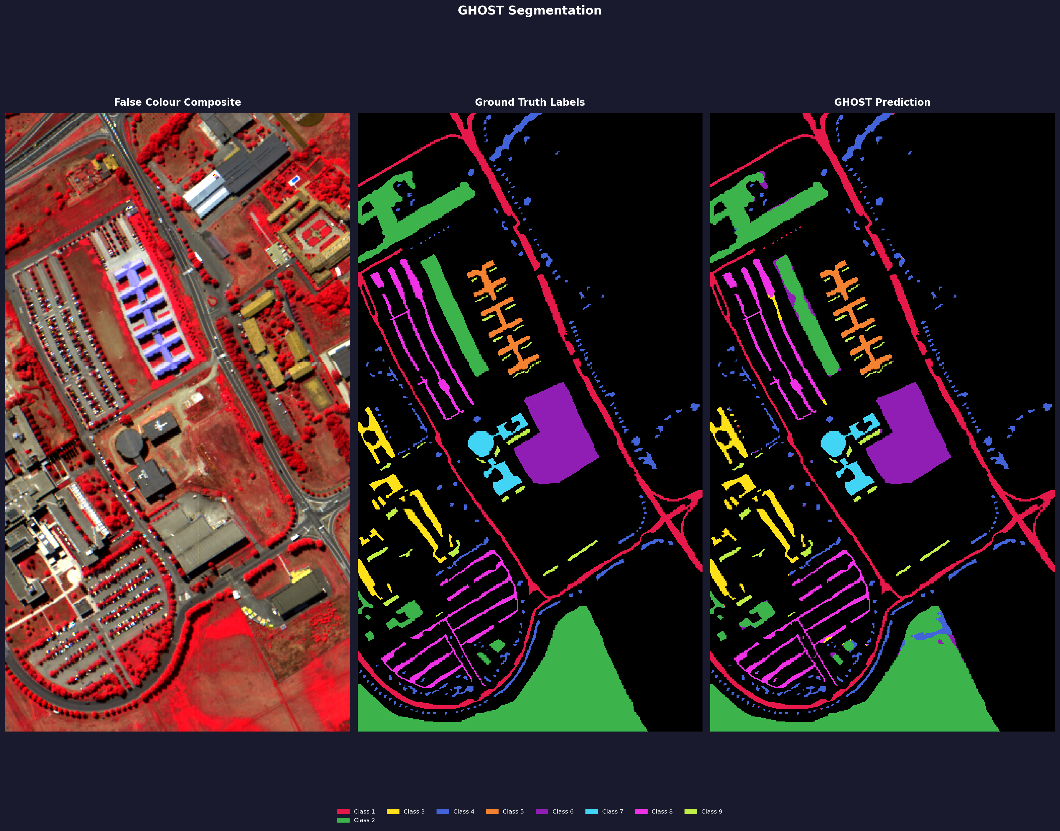
Pavia University

103 bands · 9 classes · Remote Sensing (ROSIS)

Metrics

Config	OA (%)	mIoU	Kappa
32 / 8	97.47	0.9531	0.9667

Config

Base / Num Filters	GPU	Time
32 / 8	Kaggle T4	7h 29m

Standard pixel-level split, seed 42, forest routing, dice loss. Ran on Kaggle free tier T4.

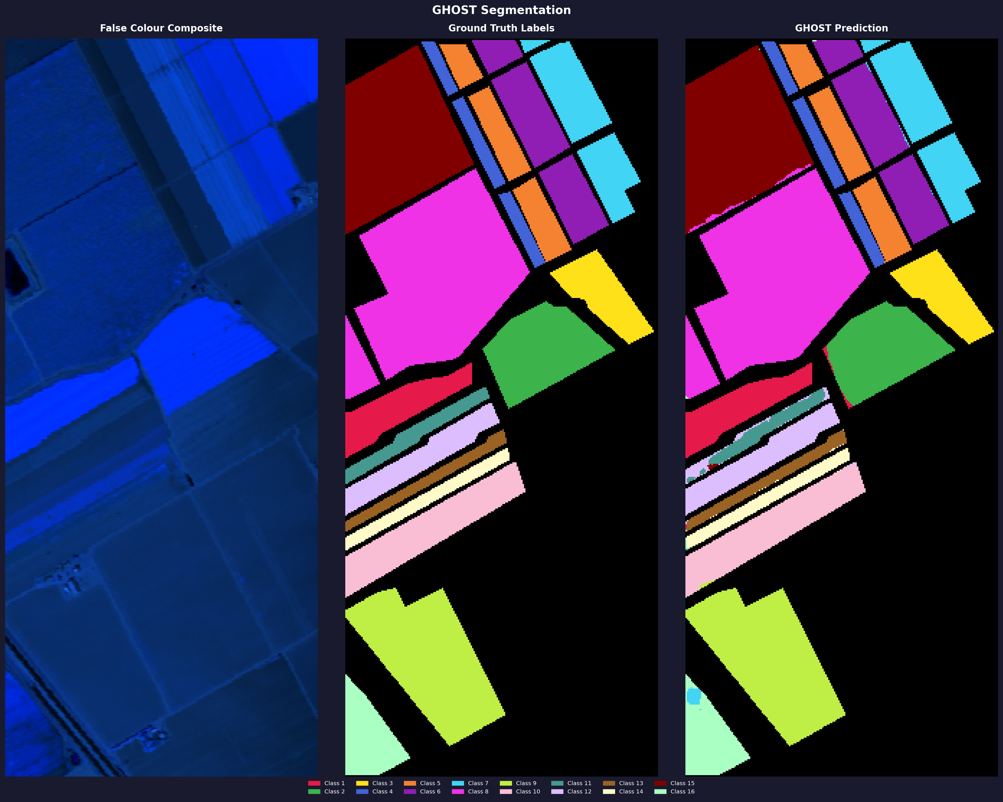
Salinas Valley

204 bands · 16 classes · Remote Sensing (AVIRIS)

Metrics

Config	OA (%)	mIoU	Kappa
32 / 8	98.69	0.9577	0.9855

Config

Base / Num Filters	GPU	Time
32 / 8	Kaggle T4	10h 51m

Standard pixel-level split, seed 42, forest routing, dice loss. Ran on Kaggle free tier T4.

LUSC (Lung Cancer)

61 bands · 3 classes · Medical Histopathology

Metrics

Config	OA (%)	mIoU	Kappa
32 / 8	99.42	0.9263	0.9876

Config

Base / Num Filters	GPU	Time
32 / 8	RTX 3050 (laptop)	1h 8m

Single tissue result only. This is from one 512×512 crop from a single patient scan — it is not representative of the full LUSC dataset and cannot be compared to published clinical benchmarks. The dataset has 60+ scans; multi-scan evaluation is a v0.2.x goal. Dataset: HMI Lung Dataset.

Mars CRISM

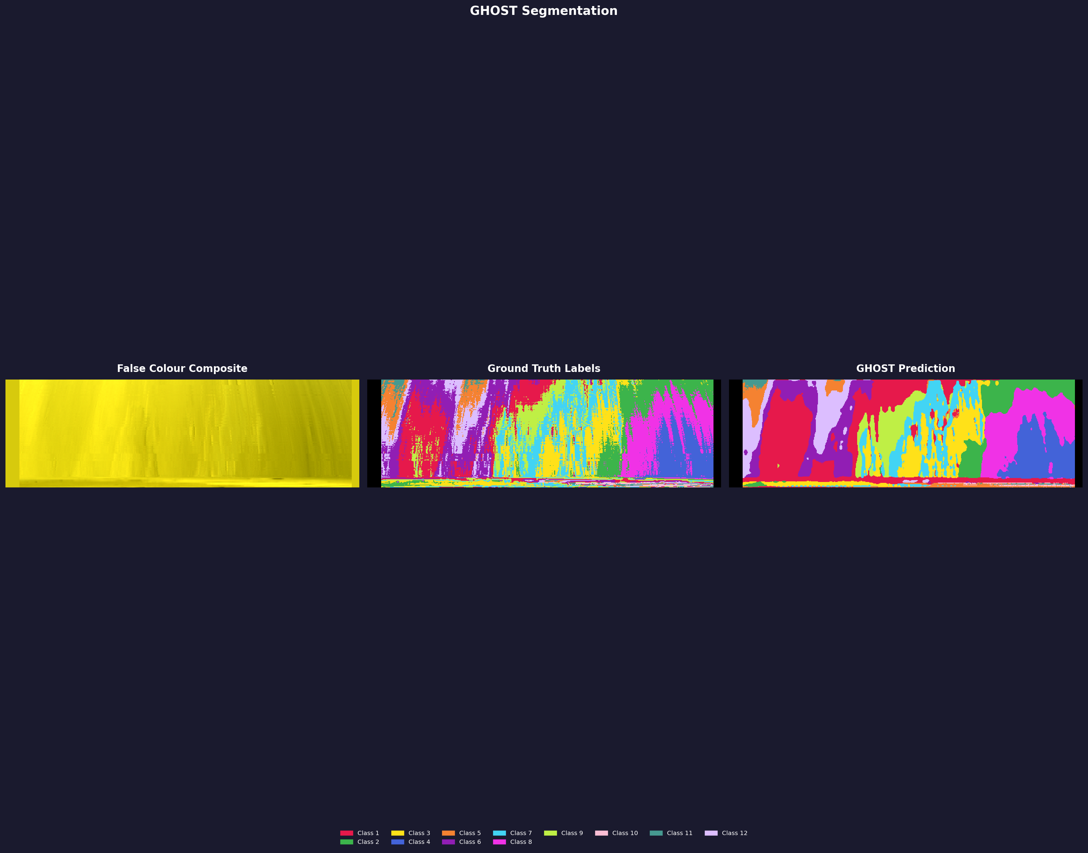
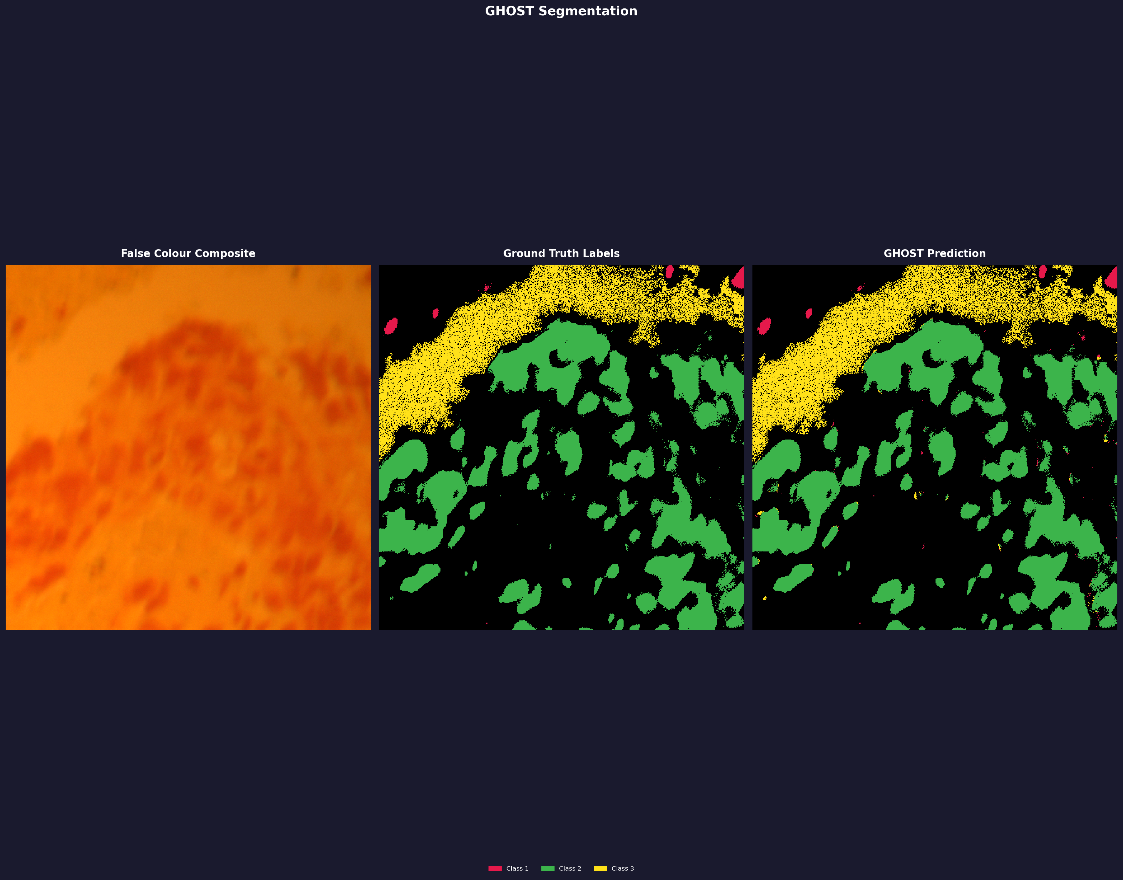
~400 bands · Mineral mapping · MRO/CRISM

Metrics

Config	OA (%)	mIoU	Kappa
32 / 8	71.70	0.5228	0.6829

Config

Base / Num Filters	GPU	Time
32 / 8	Kaggle T4	6h 44m

Quantitative results pending a clean run. The CRISM ground truth annotations are extremely sparse and noisy — the labels themselves are grainy, which drags down the numbers even when GHOST produces a visually smooth and consistent segmentation. The image shows what GHOST predicted. Annotation quality is a known limitation of this dataset. More details once I have a proper evaluation set up. Dataset: NASA MRO/CRISM.

Why no comparisions ?

Every published HSI method I'm aware of — including v0.1.x of this project — relies on spatial context. U-Nets, 3D CNNs, hybrid architectures: they all, to varying degrees, learn where things tend to be in a scene alongside what they look like spectrally. That's why they get high numbers on benchmarks. It's also why they don't generalize across scenes.

Comparing GHOST v0.1.x against those methods would be comparing like-for-like on a metric that doesn't test the actual thesis. The numbers might look competitive. They'd mean nothing.

The comparison that matters is this: does a spectral-only model, with no access to neighboring pixels at any stage, hold up across scenes it has never seen? That's the question v0.2.x is trying to answer. That's the benchmark worth publishing. Until that result exists — properly evaluated, with ablation studies, on multi-scene data — putting up a table of same-scene OA scores against the literature would just be adding more noise to a space that already has plenty of it.

Then why publish at all?

Because three of the four things GHOST set out to do are already done.

The same binary, unchanged, has segmented an AVIRIS remote sensing scene with 200 spectral bands, a lung cancer histopathology slide with 61 bands, and a Mars CRISM mineral map with ~400 bands. No format-specific code paths. No domain-specific preprocessing. No configuration changes between them. Data agnosticism, band-count agnosticism, sensor agnosticism — all three work.

Most HSI research treats remote sensing and medical imaging as entirely separate problems. GHOST doesn't. That's not nothing, even before cross-scene generalization is solved.

The fourth objective — true spectral-only generalization — is the hard one, and it isn't finished. But the foundation it needs is already there.

Architecture.

What's in the current build, and what's being redesigned.

Preprocessing

Continuum Removal (Simplified)

A straight line is drawn from the first spectral band to the last, and the spectrum is divided by it. This removes the overall reflectance slope caused by illumination angle and atmospheric scatter — the dominant non-chemical variation in raw HSI data.

It's a reasonable starting point. The main limitation is that it doesn't normalize absorption features relative to their local context — a deep absorption dip sitting next to a tall reflectance peak and the same dip next to a short peak can look different in the output, even though the underlying chemistry is identical. Full convex hull continuum removal (planned for v0.2.x) handles this more properly.

Feature Extraction

Spectral 3D Conv Stack

Three sequential 3D convolutions with a (7, 3, 3) kernel — 7 bands deep spectrally, 3×3 spatially. The model learns that nearby spectral bands correlate with each other, and that nearby pixels tend to share materials.

The spatial component is both a strength and a problem. It captures local context, which helps within a single scene. But it also means the model is learning where things tend to be, not just what they look like spectrally. That doesn't transfer between scenes. This is one of the main things being removed in v0.2.x.

Attention

SE Attention Blocks

Squeeze-and-Excitation blocks learn a per-channel importance weight. A global average pool reduces each feature channel to a scalar, a small two-layer MLP predicts a weight between 0 and 1, and that weight is multiplied back into the channel. The network learns to suppress less useful channels and emphasize the ones that matter for the current input.

Lightweight and effective. No major issues with it — the spirit of per-channel weighting carries into v0.2.x implicitly through the dilated ResNet encoder.

Spatial Context

U-Net Encoder–Decoder

A standard 4-level U-Net with skip connections. The encoder downsamples through MaxPool2d, the decoder upsamples via transposed convolutions, and skip connections link matching levels. Channel progression: f → 2f → 4f → 8f → 16f.

This is where most of the learning happens in v0.1.x — and also why the model doesn't generalize across scenes. The U-Net effectively learns "where things are" in the training image. Corn fields tend to appear in certain shapes, urban structures have spatial patterns. None of that is true in the next scene. That's the thing I'm trying to remove entirely in v0.2.x.

Core Engine

Spectral Partition Tree (SPT)

Previously called RSSP (Recursive Spectral Splitting with Parallel Forests), SPT is a divide-and-conquer strategy over the class set. It builds a binary tree where classes are recursively split based on SAM (Spectral Angle Mapper) distance — spectrally similar classes are grouped together and handled by specialist ensemble models.

The reasoning: asking one flat model to separate 16 highly imbalanced classes is hard. SPT lets one model split broad groups (vegetation vs. minerals), then separate specialists handle the hard within-group cases (corn subtypes, mineral variants). Each leaf ensemble focuses on a smaller, more tractable problem. In practice this helps a lot with class imbalance.

The SPT logic is unchanged in v0.2.x — only what lives inside each tree node changes.

⚠ Broken

SSSR Router (Experimental)

SSSR (Spectral State-Space Router) was an attempt to replace hard argmax routing between tree nodes with a learned spectral state-space model — differentiable, soft routing probabilities instead of hard decisions at each branch.

In practice it doesn't work. Ensemble routing (--routing forest) outperforms it in every configuration I've tested. The SSM pretraining adds significant wall-clock time, and the routing improvement simply doesn't materialize. The code is currently broken and not recommended.

It may be revisited in v0.1.7+ or rethought entirely for v0.2.x. For now, always use --routing forest and set --ssm_epochs 1 to skip SSM pretraining entirely.

v0.1.x

Known Limitations

Spatial dependence: The U-Net backbone processes neighboring pixels together. A model trained on one scene cannot reliably segment a different scene — it has learned spatial patterns alongside spectral ones.
No transfer learning: Each new dataset requires a full training run from scratch. There's no way to reuse weights from a previous run in any meaningful way.
Single scene only: Training and inference must be on the same scene, or at very minimum the same sensor under near-identical conditions.
SSSR router is broken: Use --routing forest. See above.

Preprocessing

Full Convex Hull Continuum Removal

v0.2.x computes the upper convex hull of each pixel's spectrum — a ceiling that touches all the local reflectance peaks. Dividing the raw spectrum by this hull normalizes every absorption feature relative to its local context. Values at 1.0 mean no absorption at that wavelength; values below 1.0 represent absorption depth directly.

This is the physically correct approach. The dip position encodes which molecular bonds are present, the depth encodes concentration, and the width encodes the type of transition. Two spectra of the same material should look nearly identical after this normalization, regardless of illumination or atmospheric conditions, because the underlying chemistry is the same.

Implementation uses Andrew's monotone chain algorithm (O(n), upper hull only) with Savitzky-Golay smoothing applied before hull computation to stop noise spikes from becoming false hull vertices. The raw spectrum — not the smoothed one — is divided by the hull, which preserves narrow real features in the output.

Spectral Encoder

1D Dilated ResNet Encoder

The core change in v0.2.x: each pixel's spectrum is processed independently by a 1D dilated residual network. There are no 2D or 3D convolutions anywhere. No neighboring pixels. No spatial context. The encoder receives one spectrum and outputs a fixed-size embedding representing its spectral fingerprint.

Dilated convolutions with increasing dilation rates (1, 2, 4, 8, 16...) give the encoder a wide receptive field across the spectral axis without any downsampling, allowing it to see both narrow absorption features and broad spectral shapes simultaneously. The architecture auto-adapts its depth and kernel size to the input band count at construction time — no manual configuration needed for different sensors.

Global average pooling at the end collapses the spectral dimension to a fixed-length vector. The MLP head classifies from this vector. That's the entire model from input to output — no spatial operations anywhere in the chain.

Classifier

MLP Classification Head

A small two-layer MLP on top of the encoder: Linear → BatchNorm → ReLU → Dropout → Linear. The non-linear hidden layer helps when the spectral embedding isn't perfectly linearly separable for very similar classes — two vegetation subtypes with nearly identical spectral fingerprints, for instance.

Each SPT node trains its own independent encoder + head pair, and each ensemble member at a node uses a different random initialization. Fully independent models, not a shared encoder with different heads. This matters for ensemble diversity — shared encoders collapse toward the same solution regardless of head initialization.

Unchanged

Spectral Partition Tree (SPT)

The SPT logic from v0.1.x carries over unchanged. SAM-based class clustering, recursive binary splitting, per-node ensemble training, soft cascade inference — all identical. The only difference is what lives inside each node: a 1D ResNet + MLP instead of 3D Conv + U-Net.

The SPT is the part of GHOST I'm most confident about. Splitting a hard multi-class problem into a hierarchy of simpler problems, with specialists for each group, seems to work well regardless of the backbone. It's a clean structural idea that I think will survive into whatever version comes after v0.2.x.

Optional

Dense CRF Post-Processing

After the per-pixel spectral classification, an optional dense CRF pass can smooth the output probability map spatially. The CRF balances two signals: the spectral model's class probabilities (unary potential) and the spatial and spectral similarity between neighboring pixels (pairwise potential). Confident predictions stay mostly unchanged; uncertain pixels near boundaries are nudged toward their neighbors.

This is the only place spatial information enters v0.2.x, and it operates on the output probabilities, not the learned features. The model's classification decisions are 100% spectral — the CRF just cleans salt-and-pepper noise from uncertain pixels. Off by default. Probably helpful for remote sensing data with large homogeneous regions; probably wrong for medical imaging where cellular-level heterogeneity is real.

Future

Self-Supervised Learning (SSL)

One chronic problem in hyperspectral imaging is labeling cost. Annotating every pixel in a scene requires domain expertise, and even expert annotations tend to be noisy and incomplete. Most benchmark datasets have only a few hundred labeled pixels across tens of thousands.

SSL is an attempt to pretrain the spectral encoder on large amounts of unlabeled HSI data using masked spectral modeling — hiding some spectral bands and asking the model to predict them, similar in spirit to BERT-style pretraining for text. The goal is an encoder that already understands spectral chemistry from unlabeled data and needs only a small number of labeled examples to adapt to a new scene or domain.

This is deferred to after v0.2.0. It requires a reasonable collection of diverse unlabeled HSI data and careful evaluation to know if the pretraining is actually learning chemistry or just memorizing sensor response patterns. It's on the radar, just not in the current build.

Roadmap

What v0.2.0 Is Actually Trying to Do

Being honest about scope: v0.2.0 is not claiming to solve HSI generalization. It's one attempt at a specific subset of it.

Spectral-only classification Every pixel classified from its spectrum alone, with no access to neighboring pixels. If it works, the model has learned material chemistry — and chemistry is the same whether the vegetation is in Indiana or Vietnam.
Native multi-format support ENVI (.hdr), GeoTIFF (.tif), HDF5 (.h5) read directly by the training and inference pipeline — no conversion step needed. v0.1.7 ships ghost convert_to_mat as a bridge in the meantime.
Multi-scene training and inference Train on 2 scenes, run inference on 10 more. The actual test of generalization: if the spectral-only approach works, the model should segment unseen scenes from the same sensor without any retraining.
Same binary, different domains Remote sensing and medical imaging on the same codebase, zero configuration changes between them. Retrain on new data, but change nothing else.

What v0.2.0 won't claim: cross-sensor transfer (different instruments measuring the same materials) or zero-shot generalization (train on crops, segment minerals without retraining). Those are harder problems that likely require SSL and sensor response function handling. They're deferred.

Why spectral context?

There's a persistent problem in hyperspectral imaging that I don't see talked about much directly: a model trained on one scene generally can't be used on another.

You train on Indian Pines and get 97% accuracy. You run the same model on Salinas Valley and it falls apart — not because the materials are different (both scenes have vegetation, bare soil, crops), but because the model learned where things tend to be, not what they are spectrally.

Current HSI methods, including v0.1.x of this project, rely heavily on spatial context. A U-Net learns that "pixels in this area tend to be corn because they're spatially clustered with other corn pixels." That pattern holds within one scene. It means nothing in the next.

What should generalize is the chemistry. Chlorophyll absorbs light at around 680 nm because of its molecular structure — that's true whether you're looking at a corn field in Indiana or a rice paddy in Vietnam. Hemoglobin absorbs differently from collagen, regardless of which patient, which hospital, which staining protocol. Spectral fingerprints are determined by molecular bonds, and molecular bonds don't change between scenes.

If a model learned to classify from spectral evidence alone — no location, no neighbors — you could train it on two scenes and use it on fifty more. That's the goal of v0.2.x: remove all spatial context from the classification loop and force the model to rely entirely on the spectrum of each individual pixel.

I want to be upfront that this is an experiment. Whether the spectral-only approach delivers on that promise is something that needs to be demonstrated, not just argued. The v0.2.x evaluation on multi-scene datasets is what will actually tell us. But the reasoning seems sound, and it's worth trying — especially since I haven't found a clean, accessible implementation of this idea elsewhere in the literature.

What makes it difficult ?

Spectral variance within groups is often larger than between groups. What this means is that if element A has absorption characteristics that vary significantly within its group, it can be difficult to distinguish it from element B, even if B has different absorption characteristics overall. If A has features between 100nm and 200nm while B has features between 150nm and 250nm, then the region between 150–200nm becomes highly ambiguous.

Beyond overlapping signatures, real-world conditions rarely give us pristine data. Variables like illumination angles, shadows, canopy geometry, and atmospheric scattering constantly distort the readings. Two identical crop fields can yield distinct spectral profiles simply because one was imaged at noon and the other at 4 PM under thin clouds.

Because of these ambiguities, current methods in the literature—just like v0.1.x of this project—take the easy way out: they lean heavily on spatial context. They operate on the logical assumption that if 10 pixels around pixel X are corn, then X is highly likely to be corn as well. Spatial architectures like U-Nets excel at learning these neighborhood patterns, effectively smoothing over the spectral noise.

But this spatial crutch masks the underlying problem. It ties the model's performance to the specific spatial layout of the training scene. When we remove that spatial safety net in v0.2.x, the model loses the ability to infer a pixel's identity from its neighbors. It is forced to confront the raw, messy chemical reality of "mixed pixels" and atmospheric distortion on its own.

Tackling these hurdles—intraclass variance, atmospheric distortion, and high dimensionality—without relying on spatial crutches is what makes v0.2.x a formidable challenge. The model has to learn the true, underlying chemical reality amidst a sea of noise. Convex Hull Continuum Removal and SPT have proven to be quite effective at learning this spectral context, but further studies are needed.

What has been achieved so far ?

The incomplete v0.2.x build has been tested on Indian Pines under a strict spectral-only regime — 100 pixels per class for training, with 40% of available pixels used for smaller classes, and zero spatial context at any point in the pipeline. The result was 92% OA. No neighbors. No U-Net. No spatial smoothing of any kind.

That number alone isn't what's interesting. What's interesting is the per-class mIoU distribution. Across nearly all classes, mIoU sits consistently around 0.7 — the model isn't carrying a few easy classes while failing silently on hard ones. The only meaningful outlier is Class 7 (Grass-pasture-mowed), which has very few labeled pixels in the Indian Pines ground truth to begin with — a data problem, not a model problem. The uniformity across the remaining classes is the first real evidence that the model is learning spectral chemistry rather than spatial habit.

This result is preliminary. The full convex hull continuum removal implementation is not fully optimized — the simpler linear continuum removal currently outperforms it, which suggests the hull computation is introducing noise rather than removing it. That needs to be resolved before any result involving continuum removal can be reported cleanly. GPU utilization is also unoptimized, which makes thorough hyperparameter sweeps expensive and slow.

The ablation studies have not been completed or documented to a publishable standard. Claiming 92% OA without showing what each component contributes — SPT, continuum removal, dilation rates, ensemble size — is a number without a story. Those studies are in progress and will be reported in full once they are. Until then, treat this as a proof of direction, not a finished result: spectral-only classification on Indian Pines is viable, and the per-class consistency suggests the architecture is learning the right thing.

I will open source the code only once ghost-hsi v0.2.x has reached a stable release, achieved better numbers and has publishable ablation studies. For more details, feel free to reach out to me at IshuIsAwake.

Start here.

Install.

Install from PyPI. Indian Pines sample data is bundled — run ghost demo to get the file paths.

$ Terminal

pip install ghost-hsi
ghost demo

Train.

Run the full GHOST pipeline with SPT. Use the paths printed by ghost demo.

$ Terminal

ghost train_spt \
  --data /path/to/Indian_pines_corrected.mat \
  --gt   /path/to/Indian_pines_gt.mat \
  --loss dice --routing forest \
  --base_filters 32 --num_filters 8 \
  --ensembles 5 --leaf_ensembles 3 \
  --epochs 400 --patience 50 --min_epochs 40 \
  --out-dir runs/my_experiment

Predict.

Run inference on the test split and compute metrics.

$ Terminal

ghost predict \
  --data  /path/to/Indian_pines_corrected.mat \
  --gt    /path/to/Indian_pines_gt.mat \
  --model runs/my_experiment/spt_models.pkl \
  --routing forest --out-dir runs/my_experiment

Visualize.

Generate a 3-panel segmentation figure: false colour composite, ground truth, GHOST prediction.

$ Terminal

ghost visualize \
  --data    /path/to/Indian_pines_corrected.mat \
  --gt      /path/to/Indian_pines_gt.mat \
  --model   runs/my_experiment/spt_models.pkl \
  --dataset indian_pines --routing forest \
  --out-dir runs/my_experiment